Analyzing results

Study runs

The left panel lists the runs from this session and your saved studies. The current run is selected automatically when you enter Analysis; “Save run” preserves it beyond the session so an existing-conditions study stays available while you test alternatives. A search field filters saved studies by name.

Charts

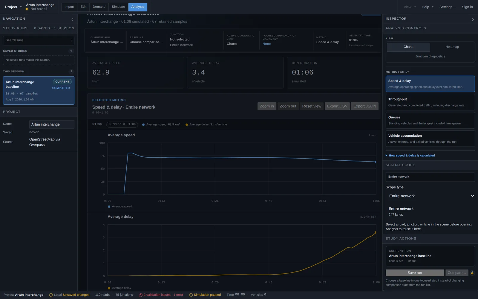
The Charts view plots the run over simulated time across four metric families — speed & delay, throughput, queues and vehicle accumulation. A time scrubber selects any retained sample, charts can be zoomed, and the data behind them can be exported as CSV or JSON.

Network heatmap

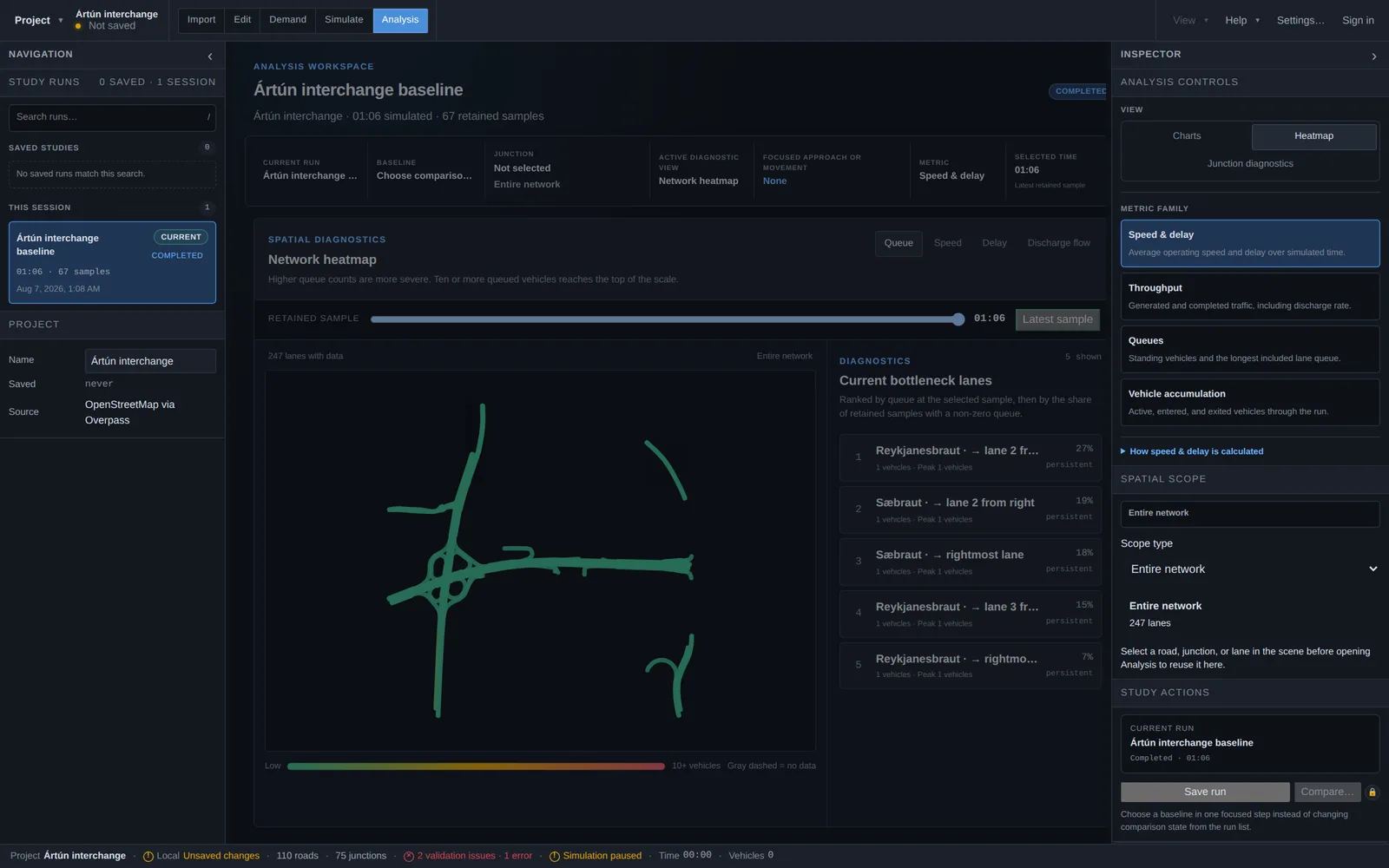
The Heatmap view paints metrics directly onto the network geometry — queue counts, speed, delay or discharge flow — at any retained sample, with a ranked list of current bottleneck lanes beside it. It is the quickest way to see where congestion forms and how far it spreads.

Level of service

The Level of service view grades every junction with recorded turning movements from A to F, the scale traffic studies and their reviewers already know from the Highway Capacity Manual. Grades come from estimated control delay — the time vehicles lose between entering an approach and clearing the junction, volume-weighted across movements and approaches, with the warm-up period excluded — using the HCM thresholds for signalized junctions and the unsignalized thresholds for priority junctions and roundabouts.

Junctions are listed worst-first with their control type, traffic volume, delay and worst approach, and each row opens the full junction diagnostics. The same grades appear as chips on the junction workspace's approach and movement tables and in its CSV/JSON exports. Grades are labeled as estimates: the methodology page explains exactly how the delay is measured.

Junction diagnostics

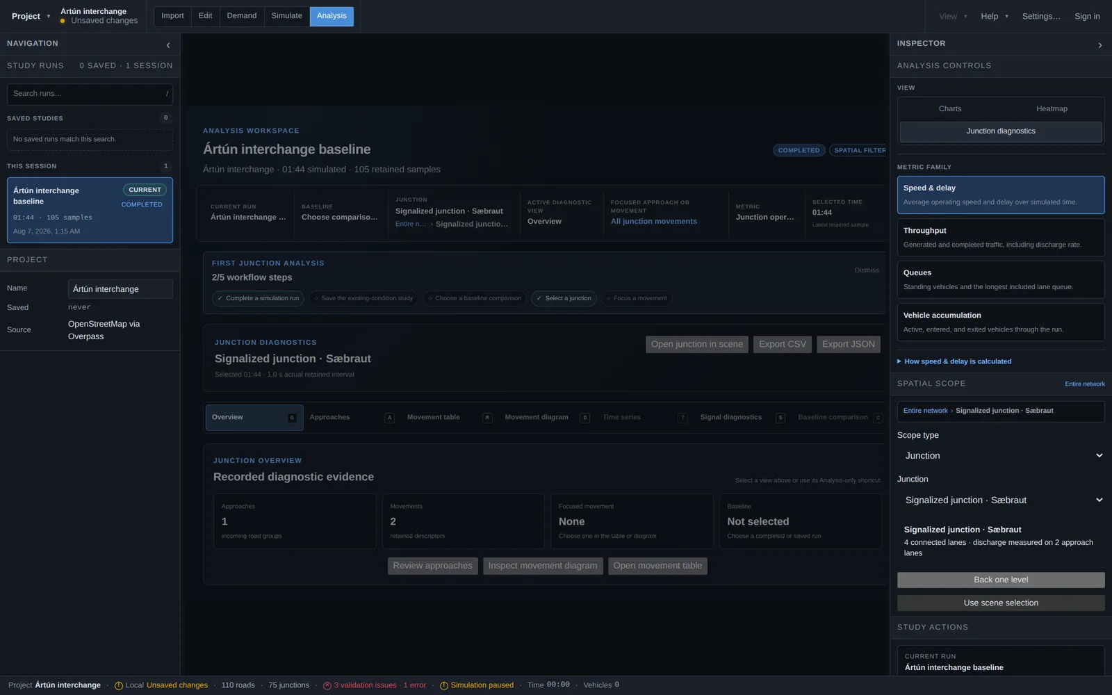
Junction diagnostics drills into a single junction: pick one via the spatial scope (or select it in the scene and press “Use scene selection”), and the workspace offers focused views — approaches, a turning-movement table, a movement diagram, per-movement time series, and signal diagnostics for signalized junctions. A five-step guided workflow walks you from a completed run to a focused movement comparison.

Comparing runs

Choose any completed or saved run as the baseline and the workspace overlays it against the current run — charts gain comparison series and junction views gain baseline columns. The deterministic engine makes these comparisons meaningful: differences come from your edits, not random variation. Spatial scope narrows any view to a road, junction or selection instead of the entire network.

Runs recorded in a scenario other than the active one are badged in the run list, and a note appears when a run's network differs from the one currently loaded — charts and totals are exact, but heatmaps and junction views are drawn against the active network.

Replications and confidence intervals

One run is one realization. The Replications view runs the current scenario many times with consecutive seeds — headlessly, in background workers at full processor speed rather than at playback speed — and reports every key figure as a mean with a confidence interval: average delay, average speed, throughput, queued vehicles, longest queue and completed trips, all warm-up excluded. Ask for a fixed number of runs, or state a target — “±10% of average delay at 90% confidence” — and the workspace keeps adding runs until the interval is that tight or a cap is reached, showing a running estimate of how many runs it will take. An optional stop condition ends each run early once every lane's queue has stayed below a chosen length for a chosen time.

Results include the statistics table, a per-run list and a Level-of-Service summary that grades each junction on its mean delay and shows the grade spread across runs (for example “C, ranging B–D”); the whole set exports as a multi-block CSV. The view warns when arrivals are set to Uniform, because confidence intervals from evenly spaced arrivals understate real variability — switch to Poisson arrivals in Simulate first. Replications are a Team-plan capability.

Comparing scenarios

The Scenarios view puts every scenario in the project side by side: one row per scenario with its latest completed run, the same warm-up-excluded key figures the Replications view uses, its worst Level-of-Service grade, and colored deltas against a reference row you choose — green where the change reads as an improvement, red where it reads as a regression. Runs that predate scenario tracking are counted but never guessed into a row; record a fresh run in a scenario after editing it. The table exports as CSV for the study report.

Raw data exports

Everything the workspace shows can leave it as data for spreadsheet analysis. The Charts view exports the full retained time series — one row per sample with per-lane columns (active vehicles, speed, delay, entered, exited, queue by lane id), per-movement columns, per-junction signal state and per-source generation. Junction diagnostics exports a multi-block CSV with approach summaries, the turning-movement table, Level-of-Service grades, baseline comparisons and observed signal cycles. All CSVs open directly in Excel; JSON variants carry the same data for scripted pipelines.