Traffic demand
Demand mode defines where vehicles enter the network, how many arrive, where they are headed and who is driving. Everything is expressed in familiar engineering terms — vehicles per hour, destination shares, vehicle classes.
Traffic sources and destinations
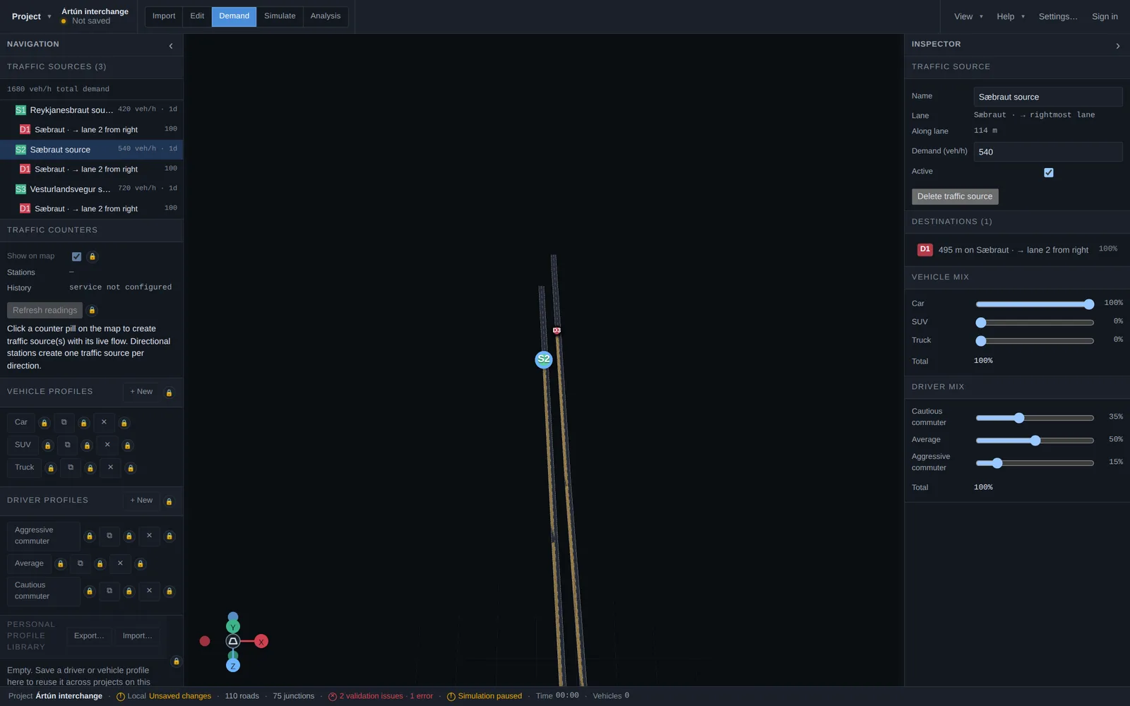
Click a road to place a traffic source on a specific lane, then click other roads to add destinations for it. Each source has a demand in veh/h and an active toggle; each destination carries a share, so one source can split its traffic 70/30 between two exits. Vehicles choose their own lanes and routes toward the destination — you specify intent, the simulation handles the driving.
The left panel lists all sources with their demand and destinations; selecting one fills the inspector with its full configuration.
Vehicle and driver mixes
Each source generates traffic from a vehicle mix (cars, SUVs, trucks by default) and a driver mix (cautious, average and aggressive commuter profiles by default). Sliders set the share of each profile per source, so a motorway source can carry more trucks than a residential one — and every share (including destination shares) also accepts an exact typed percentage next to its slider, with the other shares rebalancing so the total stays 100%.
Profiles themselves are editable: vehicle profiles define physical characteristics, driver profiles define behavior parameters used by the car-following and lane-change models. You can create new profiles, duplicate and adjust existing ones, and save favorites to a personal profile library that can be exported and imported across projects.
Seeding demand from traffic counters
Where public traffic-counter networks are available, Demand mode can show measured flows directly on the map: enable “Show on map” under Traffic counters and click a counter pill to create traffic sources carrying its measured flow — directional stations create one source per direction. Supported networks currently cover Iceland (Vegagerðin and City of Reykjavík), the Netherlands (NDW), Finland (Fintraffic), France (Bison Futé) and California (Caltrans Traffic Census — annual AADT averages rather than live readings); the source used is chosen automatically from the import area.
Live counter readings are a paid-plan capability, and historical counter data (the demand “time machine”) is available on Team and Enterprise plans. The time machine offers the last hour, day and month at increasing bucket sizes, every day's peak, and a Pick day tab with a calendar: choose any day and hour to build demand from that reading. Hourly readings are kept for the last 30 days and the daily peak indefinitely; the archive accrues forward from when polling began, so there is no backfill of earlier years.
Generating demand from counters automatically
Instead of converting stations one by one, “Generate demand from counters…” under Traffic counters builds a complete origin–destination pattern for the whole import area. Every station inside the area becomes a traffic source per counted direction; stations whose lane leads straight out of the network lend their count to that exit; destinations are the network's exits. A gravity model seeds the trip table over route distance and Furness balancing scales it so each source sends its counted volume and each counted exit attracts its counted volume, with uncounted exits sharing the remainder. Every destination is checked for reachability with the same routing the simulation uses.
The result is reviewed before it lands: a dialog lists each source with its lane, volume and destination count, plus every assumption the heuristic made — stations too far from an imported road, stations without a current reading, totals without a direction split, and mid-network stations whose counts include through-traffic. Apply replaces earlier counter-generated sources (manually placed sources are kept) as one undo step, and the generated sources stay fully editable afterwards. It is explicitly an estimate: treat it as a starting point that reproduces the counts, then refine.
Scenarios
A project can hold several named scenarios — a baseline plus alternatives — managed from the Scenarios panel at the top of Demand mode. Each scenario has its own demand (sources, destinations, mixes, seed, warm-up) and its own closures: closing a road in one scenario leaves the others untouched, and a closure made in the baseline is inherited by the alternatives, which may reopen it locally. “New scenario from active” duplicates the current scenario as a starting point; switching is one click, and the status bar shows which scenario is active whenever there is more than one.
The road network itself belongs to the baseline. Structural edits in an alternative — moving geometry, changing a junction, adding a lane — give that scenario its own copy of the network the moment they happen (the panel marks it “own network”), so alternatives can carry real design changes, not just demand. If the baseline network is edited later, such a scenario is flagged “base changed” with an option to duplicate it onto the current base. Every recorded run remembers which scenario produced it, which is what makes the scenario comparison in Analysis possible. Multiple scenarios are a Team-plan capability.